Creating a Basic Table

Now the fun begins!

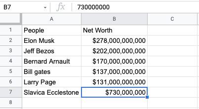
Go ahead and start typing out some information like this below. It’s good to include words in one column and numbers in others to see how they look. The keen-eyed amongst you will have spotted that words align to the left of a cell, whereas numbers align to the right.

There is a good reason for this; it makes sense when considering words as we read and write from left to right; otherwise, it would look odd. When it comes to numbers, you can visualise the size of a number better when it’s right-justified.

I’ve just formatted column B to show these numbers in USD to put this into perspective. You can see the number in the highlighted cell (B7) is much smaller than the others, and that’s where this right alignment comes into play.

Alignment

There are a few ways to change the alignment of text and numbers in a cell. First, with the cells highlighted that you want to change, click on the format option in the menu and choose Alignment.

Now you can choose to format any text that’s highlighted to the left, centre or right justified, plus you can also position the text to the top, middle or bottom of the cell if that’s what you want to do.

You’ll notice the shortcut keys next to the text in the menu, which is another quick way to change this.

Finally, you can use the alignment tool in the formatting ribbon to align the text horizontally.

The icon next to this will align the text vertically in the cell, either top, middle or bottom.

Formatting Numbers

To set the format for the numbers it’s a similar action. With the cells highlighted that you want to format, click Format in the menu and then choose Number to see a list of formatting options.

The quicker way is to choose the 123 dropdown icon from the formatting ribbon, which will show you the same menu and set of options.

I used USD as the list of people in this example shows their net worth in US dollars, but you can choose any currency you want; just look for custom currency right at the bottom of this dropdown list.

If you choose the Accounting option, you’ll get the amount shown with two decimal places by default. You can hide these by clicking on the Decrease Decimal Places icon a few times or put them back again by clicking the Increase Decimal Places icon next to that.

We’ll add final touches to make this look more like a table. First, we’ll make the heading row bold and centre aligned. You can use the shortcuts Cmd+B for bold on a Mac or Ctrl+B on a PC. We can also use Cmd+Shift+E or Ctrl+Shift+E to make the text central.

Lastly, add a border line under the heading; choose the border option from the formatting ribbon and the lower borderline. Check out this post for 6 Tips for Formatting Headers in Google Sheets

Here’s the final table. It’s no masterpiece, but it’s a starting point for getting to grips with the formatting options at your disposal.

Happy table creating!