How to Remove Duplicate Rows in Google Sheets

Removing duplicate entries in Google Sheets can be a time-consuming and tedious task. Fortunately, there’s a way to streamline the process with formulas. With a few simple formulas, you can quickly and easily remove duplicates from your data.

When a record appears multiple times in your data, it is known as a duplicate. Identifying duplicates in Google Sheets is crucial before commencing any data analysis, as they can create significant issues.

In this article, we will discuss how to remove duplicates in Google Sheets using formulas.

Before getting started, it’s important to recognise that Google Sheets formulas don’t always recognise duplicate entries. In other words, if two entries are identical but have different capitalisations or spacing, the formulas won’t recognise them as duplicates. Therefore, it’s important to make sure that your data is clean before attempting to remove duplicates with formulas.

We can use two main formulas in Google Sheets to remove duplicates: UNIQUE and QUERY. Let's take a closer look at each of them.

UNIQUE Formula

The UNIQUE formula in Google Sheets is a powerful tool to help us remove duplicates. It works by identifying unique values in a range of cells and returning them in a new range. Here's how we can use the UNIQUE formula to remove duplicates:

1. Select the range of cells that contain the data we want to remove duplicates from.

2. In an empty cell, type the following formula:

=UNIQUE(A2:B11)

- replace "A1:B11" with the range of cells you want to check for duplicates.

3. Press Enter to run the formula.

4. The result will be a new range of cells containing only the unique values from the original range.

You can see the new range in columns C and D only has 10 rows of data, vs 11 rows in the original dataset in columns A and B. The duplicate entry of Olivia Patel on row 10 was removed, which pushed James Garcia up one row.

QUERY Formula

The QUERY formula in Google Sheets is another tool that can help us remove duplicates. It works by filtering data based on specific criteria. Here's how we can use the QUERY formula to remove duplicates:

1. Select the range of cells that contain the data we want to remove duplicates from.

2. In an empty cell, type the following formula:

=QUERY(A1:B11,"SELECT A, B, COUNT(A) GROUP BY A, B LABEL COUNT(A)'Count'",1) 

- replace "A1:B11" with the range of cells that you want to check for duplicates. You will also need to adjust the other references to these columns within the query.

3. Press Enter to run the formula.

4. The result will be a new range of cells containing only the unique values from the original range, plus an extra column to show you which values appeared more than once.

Using the Google QUERY function would only work in a scenario like this if we could include the GROUP BY clause to allow us to group instances found in columns A and B together.

This is possible by adding an aggregated column, which in this example was COUNT(A) ~ This just counts all instances of data found in column A. Aggregating any data allows us to group by any other data, with the added bonus of being able to see which rows in the data were duplicated.

This QUERY function can be broken down into 3 parts to understand what's happening.

1. data - The range of cells to perform the query on. In this case, the range was A1:B11
   

2. query - The query to perform, written in Google Visualisation API Query Language. The whole query was "SELECT A, B, COUNT(A) GROUP BY A, B LABEL COUNT(A)'Count'" This can further be broken down as follows:
   

   1. columns SELECT A, B, COUNT(A) - This tells the query which columns to return, including our aggregated pseudonym column COUNT(A), to show how many duplicates were found. This column doesn't actually exist, but we created it here.

   2. grouping GROUP BY A, B - This allows us to filter out the duplicates by grouping the data together. You can only group by real columns, not aggregated pseudonym columns.

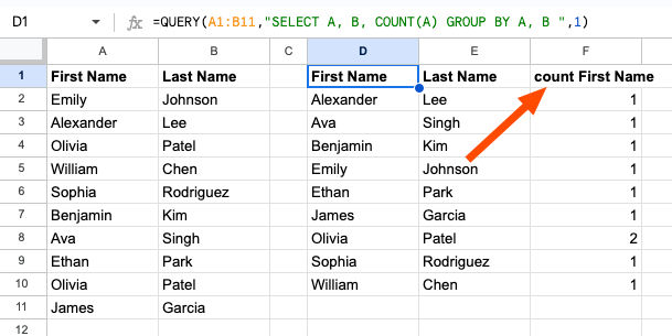
   3. labelling LABEL COUNT(A)'Count' - This simply allows us to rename the third column header to 'Count'. Without this part, the column header would be - count First Name, which looks ugly but is entirely possible. (See image below)
      

3. headers - [optional] - The number of header rows at the top of 'data'. If omitted or set to -1, the value is guessed based on the content of 'data'. This was set to 1 for this query, but it could have been omitted entirely.

The query without the label would be as follows:

=QUERY(A1:B11,"SELECT A, B, COUNT(A) GROUP BY A, B ",1)

Conclusion

Removing duplicates in Google Sheets is a common task that can be easily accomplished using formulas. The UNIQUE and QUERY functions are powerful tools that can help you to filter data and identify unique values. By using these formulas, you can save time and ensure that your data is accurate and consistent.