SUM Function

The logical step to using spreadsheets beyond just somewhere to hold some information or store lists etc. is to venture into using formulas or, more accurately, functions to gain valuable insights and ultimately save you precious time.

The most fundamental function is arguably the SUM function, which simply returns the sum of a series of numbers or cells. We’re going to dive in and take a look at how this works.

Basic methods

The most straightforward way to sum a range is to highlight the cells you want to sum up, then click on the explore icon in the bottom right-hand corner of the sheet.

You’ll see various options, but all you need to do is click on the SUM result and drag this over to where you want to see the total in the table; in our case, cell B8.

It’s that simple, but if you want to see what’s going on, just click on the B8 cell to look at the formula inside it. We’ll get into this in more detail later.

Another easy way to sum up a range of cells is to highlight the range as before but now click on the function icon on the far right of the formatting ribbon, then choose SUM.

This will complete the function for you; all you need to do is hit enter to accept it. It doesn’t get any easier than that!

The downside is that Google will place the function where it fancies; unfortunately, you don’t get to choose.

Okay, so that’s the easy way, and it’s definitely an excellent way to start working with formulas. Still, you’ll quickly realise that although it’s easy, it’s not necessarily the fastest way to achieve what you want, and it has its limitations, so let’s explore other ways of getting there.

Standard methods

Using this basic table below, we’re going to sum each column from January through to April with just a few clicks.

You can see I’ve simply typed equals ‘=’ in cell B8, and immediately Google suggested the SUM function, which is really helpful. This is the Google Explore AI at work here; it’s taken an educated assumption that it’s the SUM function we need, and it’s right, so all we need to do is either click on this pop-up or hit the tab key to select it.

Sometimes Google isn’t quite so forthcoming with its AI suggestions, in which case you’ll need to do a little bit of work, but most of the time, it’s pretty good.

You can see in the example below that I just typed =sum this time, and we actually have two options to choose from. Both will give the same results, but the first will require slightly less effort.

You can see it shows the predicted range, SUM(C2:C7), but the one beneath this just shows SUM.

If you choose the first one, Google will complete the formula for you, assuming the predicted range is correct. However, be careful, as Google occasionally gets it wrong, so it’s worth checking.

The second option (SUM) allows you to select the range you want manually. All you need to do is click on the first cell in the range you want to sum and hold the click down, then drag to the last cell in that range; now, you can let go of the click. It’s also possible to type the sum range out; you don’t have to click and drag.

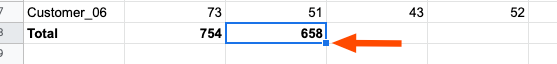
When you want to sum a range, you need to state the first cell in the range and the last cell separated by a colon ‘:’, for example, C2:C7. The complete formula can be typed like this =SUM(C2:C7). You can even see the sum of these numbers before you’ve even hit enter, which is convenient (658).

You’ll notice that after the word SUM in the function, there is an opening parenthesis ‘(‘ the range needs to sit inside an opening and closing parenthesis to work. So to finish this, you should close the parenthesis and hit enter. It’s good practice to get into this habit. But you can cheat and hit enter without the closing parenthesis. Google will figure this out.

With basic functions like this, it’s OK to take these shortcuts, but trust me, when you start adding more complexity to formulas, Google won’t be quite so helpful, so it’s a good idea to keep track of your parenthesis.

That’s pretty much all there is with the sum function, but it’s worth pointing out some tips and tricks or best practices that I’ll go over further down, so read on, as this will come in handy when setting your tables up.

Function Helpers

It’s also worth noting that if you need some help when entering your functions, you can always just click on the function name within the cell (In our case, SUM) to bring up the help icon for that particular function. Of course, this works with every function in Google too.

When you click this little blue question mark, the help pane will open up to explain that particular function. In addition, it will give you an example and the option to click the learn more link to the Google Help Centre.

Finally, to finish summing all columns in this table, we can just click and hold the little blue square and drag this across to column E to complete all sums.

We could have done this on the B8 cell, in which case it would have been two or three clicks to get all sums for Jan, Feb, Mar and Apr columns.

If you’re typing your values into a calculator and then manually entering the result into a cell, this could be a real-time-saver for you, so what are you waiting for, give it a go; you’ll be amazed how easy it is!

Best Practices

One vital thing most people overlook when creating data tables is the position of a total within the table. This should be given some thought since you might want to add more data later, and it would be a real nuisance to move things around retrospectively. Therefore, I would advocate putting your total at the very top of the data and adjusting the formula slightly to take into consideration all rows, even if they don’t have any values in them right now.

You’ll see in the example below that I have added a few extra rows above the table and changed the formula from =SUM(B5:B10) to =SUM(B5:B).

Dropping the last row number (10, in our case) tells the formula just to sum all rows right to the bottom of the sheet. This is useful as you can now just add in more data at the bottom of the table, for example, in row 11, and the formula will take this into account without you having to change anything.

This should cover most cases for the simple SUM function. You may have heard of other SUM functions like SUMIF, SUMIFS and SUMPRODUCT; we’ll dive into these functions in another lesson. These are definitely worth learning as they will unlock even more opportunities and valuable insights into your data.

Happy Summing!